Estimation of potential lost sales in retail networks of high-value substitutable products

Knowledge of products’ demand is the cornerstone of many tactical and planning decisions in supply chain systems, such as supply planning, assortment planning, inventory management, and production and logistics planning. Unfortunately, this knowledge is not always available, and it is most often costly and challenging to acquire it through field data collection. In the absence of accurate information about product demand, many firms use sales data instead of product demand for forecasting and planning. But sales data does not necessarily reflect the products desired by customers, as the purchased products may have been the result of stockout substitutions.

Customer substitution, induced by incomplete product availability, causes unrealistic inflation in sales of products that are usually available in stock. This is because these products might recapture demand for out-of-stock products. Consequently, sales of products with poor stock availability might underestimate demand for such products. Moreover, sales data does not present any information about lost sales caused by incomplete product availability (i.e., unsatisfied customers).

One solution to this problem is to estimate product demand analytically. Analytical models can provide probabilistic One solution to this problem is to estimate product demand analytically. Analytical models can provide probabilistic estimates for product demands that are well suited for scenario planning and simulation study of supply chain systems. In a paper that Benoit Montreuil and I published in IISE Transactions, we proposed a new technique to estimate product demands in a multi-store retail network using only product daily inventory in retail centers and product similarities.

Algorithm overview

As synthesized in Figure 1, our approach consists of three steps:

1. Using only past sales and daily inventory log data, we first identify all potentially desired products for a sales transaction for which demand would result in substituting to the sold products. The list consists of all out-of-stock products for which the sold product is a satisfactory substitute. For example, if a sale transaction shows P1 has been sold on day 2, we find all out-of-stock products on day 2 for which P1 has been a satisfactory substitute; hence, demanding these products could result in selling P1. These are potentially desired products for a sales transaction. Once we have the list of eligible products, we compute the “expected sales shares” for each product in the list based on their similarity to the sold product. Indeed, we split one sale credit among these products based on their similarity to the sold product. This is to account for potential stockout-based substitutions. The sum of the expected sales shares across all potentially desired products of a sale transaction equals one. The expected sales shares of a product across multiple homogenous retailers are used in the subsequent steps to estimate customer arrival rates for the product.
2. We then identify unavailable products for which potential demand could not be fulfilled with either an exact match or a satisfactory substitute. These unavailable products induce lost sales, and we refer to them as “unfulfillable” products. We also count the number of days in a month that a product has been unfulfillable in a retail center. Any demand for an unfulfillable product during this period turns to a lost sale.
3. Using the “expected sales shares” that we computed in step 1, we estimate customer arrival rates per month for each product in a retailer while considering retailers’ market sizes. In simple words, multiplying the customer arrival rate of a product by the period that it has been unfulfillable produces the expected lost sales for the product.

Model Validation

We validated the model by simulation analysis and field data collection for a case of recreational sport vehicles. In the simulation analysis, we used the model to estimate realized product demand in the simulation. We found that the model was twice as accurate as the sales data in estimating product demands. The models’ average MAPE in estimating product demands was about 23% across more than 60 studied products, while the average MAPE of the sales data was about 46%. We also found that sales data tends to underestimate demand for products. Figure 2 compares model estimates with actual demand and sales in simulation. As the Figure presents, the sales data underestimated demand for 59 products out of 63, while the model underestimated demand for 27 products. This metric is very important because demand estimates are used for future demand forecasts. Therefore, underestimations are propagated into the future predictions and cause inventory shortage and consequently lost sales. The magnitude of the model’s underestimates was also smaller than that of the sales data. The model underestimated about 8% of the total demand, while the sales data underestimated about 40% of the demand.

Implementation

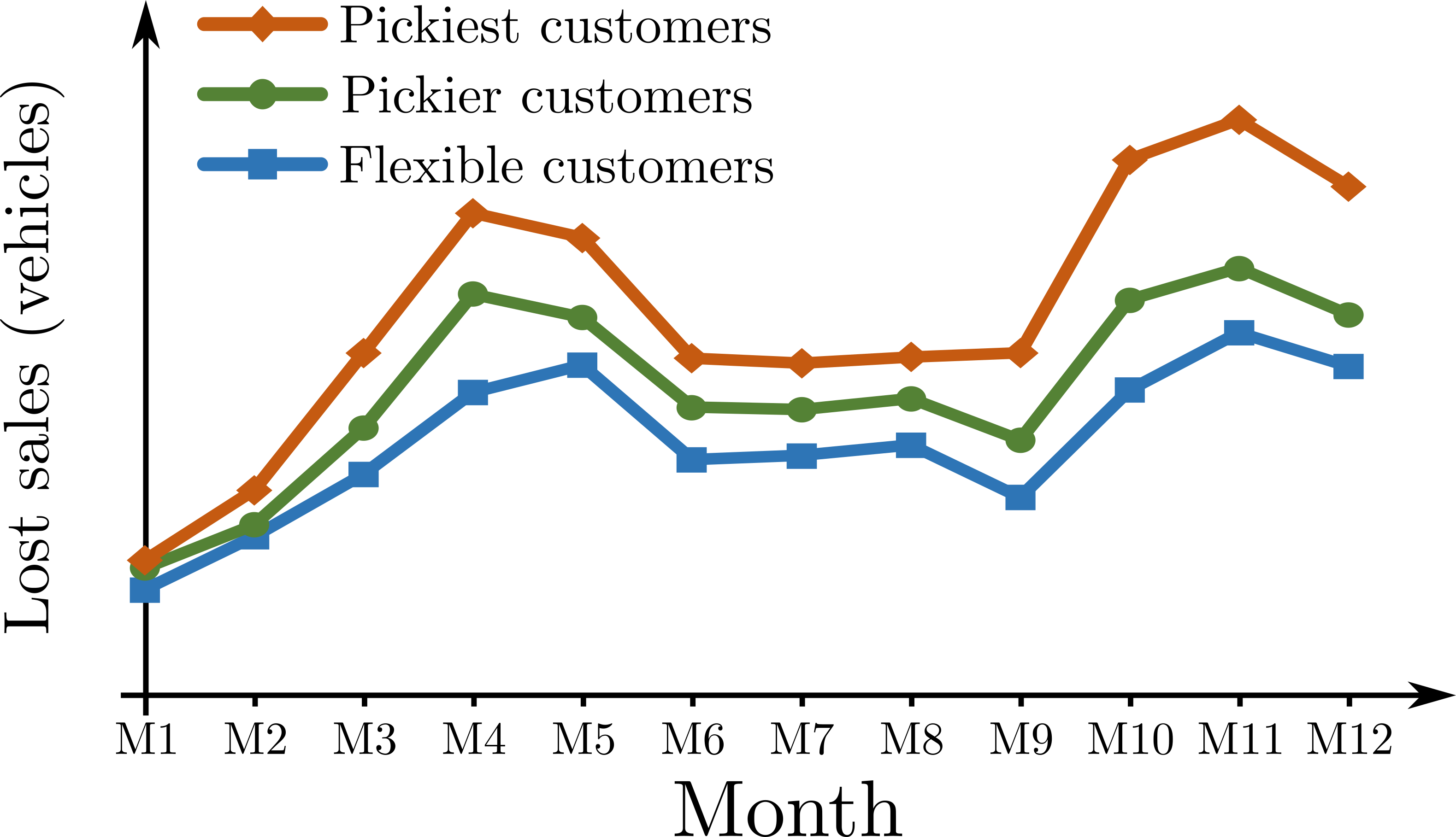
We used the model to estimate lost sales and product demand in more than a thousand dealerships of a recreational vehicle manufacturer in North America. Our analyses demonstrated that the actual sales data considerably under- or overestimate demand for most products depending on the combination of factors such as product availability, sales, and retailer market size. Our case study showed that significant supply-based lost sales and customer compromise (i.e., product substitution) occur in large dealership networks. Even with almost steady product availability, a firm may incur massive lost sales during peak demand periods. Figure 3 compares sales, estimated lost sales, and the average product unavailability in the retail network of our partner company for one year. The estimated lost sales in months M9-M12 are higher than the rest of the year, while the average product unavailability is smaller in those months (mainly because of seasonal demand). This shows a dynamic inventory management system targeting higher product availability, notably in high-demand seasons, across the entire retail network may enable a firm to reduce lost sales and product substitutions.

• 

• 

• 

For more details about the proposed approach and the case study, please see the paper. You can download it from the journal website using this link or download it directly from here. Your comments and thoughts are greatly appreciated.